Recall that in lesson 11 we saw how the set of fractions (which we denoted by FRAC) is so extremely infinite. In particular, we had “infinitely many infinities” due to the fact that between any two fractions there are infinitely many fractions, and between any of those fractions there are again infinitely fractions, and so on, forever. Moreover, the initial two fractions that we chose in this process could have been any of the infinitely fractions that exist! In this sense, FRAC appears to have “infinity times infinity” elements. Of course, the notion of “infinity times infinity” is not yet well defined, because the only infinity that we’ve defined is “infinity type 1”, which is the infinity corresponding to the set

This lesson will be devoted to showing that this vague idea of “infinity times infinity” is in fact the same as infinity type 1. In other words, we’ll find a bijective function from 


The reason why we have to get more creative is relatively easy to see. In the function from 

The problem with FRAC is that there is no meaningful order to them. Given two distinct fractions we are of course able to say which is bigger, but suppose that you give me a fraction and ask me what the “next biggest” fraction is. I would quickly respond by saying that your question is impossible to answer because, as we’ve seen, any fraction I were to say would in fact have infinitely many elements between it and the fraction you gave me, and thus surely couldn’t be the “next largest fraction”!
Therefore we can see that there will be no nice and obvious function between these two sets, and that is why we need to get creative (which isn’t the end of the world). Let us now construct this function. We will in fact only construct a function from the even elements of A to the positive elements of FRAC (recall that fractions can be positive or negative), and once we’ve done this it will be obvious that we can finish the job by sending the odd elements of A to the negative elements of FRAC in the exact same way.
We begin by recalling the following two facts. Firstly, we recall that every fraction is nothing but “some whole number upstairs, and some (non-zero) whole number downstairs”. Implicit in this statement is the fact that any whole number is itself a fraction merely by putting “1” downstairs. Secondly, we recall that 


Using the first fact as motivation, we construct an infinite chart where positive whole numbers go across the top and down the left (see figure 1). We then call the positive whole numbers across the top “numerators” and those going down the left “denominators”. Note that this chart goes infinitely far in both directions, so that it includes all of the positive whole numbers on each axis. The reason we call the numbers on the top “numerators” and those on the left “denominators” is clear: the number that goes in the corresponding square on the chart is that fraction which has its column’s “numerator” as the numerator, and its row’s “denominator” as its denominator. Note that in the figure I abbreviated “denominator” by “denom”. Clearly figure 1 only shows a small portion of the entire infinite chart, primarily because it would take me too long to write out the whole thing!

Figure 1: Infinite in both directions to cover all the positive fractions
The important thing to note about this chart is that it includes every positive fraction, seeing as it contains every possible combination of “numerator” and “denominator”, so long as we limit ourselves to the positive ones. Sure, there are some duplicates in the chart, since 


Now all we do is take the even elements of
Thus, we simply define the function from the even elements of A to this chart in the following way. Assign 2 in A to the top-left-most element in the chart (which is 


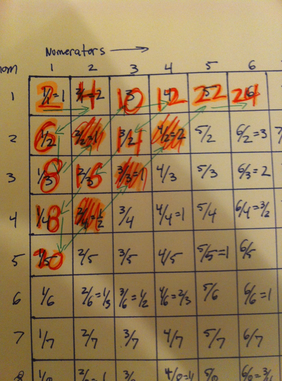
Figure 2
Now to finish the map from A to FRAC, we simply make another chart with all of the negative fractions and assign the odd elements of A to these fractions in the exact same way that we have for the positive fractions and even elements of A.
And with that, we’re done! We have successfully tamed the wild infinities that exist in FRAC and shown that FRAC is really “the same infinity” as 
Note that this function we’ve constructed is in no way “nice”, meaning that it does not have a nice pattern to it. If we call this function from A to FRAC “F”, then we see that 


We must indeed go on to the next lesson, where we finally see a brand new infinity!

Thanks for this great explanation, but the chart about fractions seems a little paradoxical.
In order to get a bijective function from natural numbers to fractions, we skip over the “duplicates” such as 2/2. My question is, what if we don’t do that? Then the resulting function would be surjective, but not injective, implying that the cardinality of fractions is less than the cardinality of natural numbers. Kindly explain this.
Hi fugitivesam, that’s a fantastic question, thanks for asking it—it goes right to the heart of what this new kind of counting (with infinite numbers) is all about. You’re right, if we don’t skip over the duplicates then we’ll hit certain fractions more than once (in fact, infinitely many times!), thus making the map surjective but not injective. But recall that it does not matter how many NON-bijective functions exist, but rather only that there is SOME bijective function between two sets for them to have the same cardinality (I’m using caps as I cannot seem to use bold here).
For example, we showed in previous lessons that the positive even numbers have the same cardinality as the positive whole numbers, and we did this by finding one bijective function between the two. Now, we could indeed define a SURJECTIVE but not INJECTIVE function from the even numbers to the whole numbers, simply by sending, say, 2, 4, 6, 8, and 10 to 1 (thus making it not injective), and then sending 12 to 2, 14 to 3, 16 to 4, 18 to 5, and so on. This isn’t injective, but it is surjective, and it’s certainly not the case that the even numbers have a larger cardinality than the positive whole numbers because there exists a DIFFERENT function that is bijective. That’s the key. As long as there is SOME bijective function, the cardinalities are the same.
Now, when we show that there is a second infinity in the coming lessons, we’re showing that there cannot possibly be ANY bijective between sets. Now here’s where the issue of surjectivity comes in. Suppose we have two infinite sets and we show that there cannot possibly be a bijective function between the two, thus showing that their cardinalities are different. How do we decide which is larger? We simply see which function can have a SURJECTIVE function from it to the other. If the cardinalities are different, only one of the two sets can have a surjective function defined from it to the other one. For example, in coming lessons we show that the real numbers have a larger cardinality than the positive whole numbers by showing that now bijective function can exist between the two. The real numbers therefore have the “larger” cardinality because we can define a surjective function from the real numbers to the natural numbers, but we can’t define a surjective function from the natural numbers to the real numbers (if we could, then we’d simply “get rid of the duplicates” and therefore have a bijective function, which we just showed was impossible).
Thus, the issue of whether or not there can be a surjective function from one set to another only arises when we’ve shown that they have different cardinalities. Then it’s used to see which has a larger cardinality. Note also that this also applies to finite sets: if the cardinalities are different, we can only define a surjective function from one to the other, and not vice versa, but if their cardinalities are the same (so that we have a bijective function between the two), then there is a surjective function both ways.
If any of this doesn’t make sense, or if it doesn’t make the issue completely clear, please do let me know!
Thanks a lot. This explanation really clicked in my head. I get it now: My statement would be valid only if there was no bijective function between them… this is brilliant. Thanks again!
No problem, glad it makes sense 🙂
TBH, I found quantumlotus’s explanation a bit hard to follow (not much experience with math, but loving the lessons so far!); so I thought I’d reply with how I picture it mentally.
I share your intuition about surjectiveness implying some sort of ‘great(er?)ness’; and that’s true as all the elements of the co-domain are mapped to by one or more elements of the domain. The important thing to note here, though, is that surjectiveness implies being ‘greater OR EQUAL TO’.
Then consider injectiveness to imply the property of the domain being ‘lesser of equal than’ the co-domain (in terms of cardinality); as for each element of the domain, there is a distinct element of the co-domain and possibly more to follow.
So I guess I’m essentially rephrasing what was said in Lesson 5: the bijectiveness implies equality as that’s the only time when something is neither lesser nor greater than the other thing (in ordered domains or w/e).
Yes, that’s exactly correct. quantumlotus (which is actually me, just an old user name haha) was just basically saying what you said only from a different starting point. Namely, if we first know that two sets are not equal, then we know that one is strictly “larger” than the other (as in cardinality), in the same way as for numbers, say. To find out which is the larger, we need to find a surjective function from one to the other, and it’s the domain of such a function that is the larger of the two. We then know that we can say this is the larger set because, by assumption, the sets don’t have equal cardinality. If it were the case that a surjective function existed “both ways”, then indeed a bijective function would exist (as you can check), and so the assumption would be wrong. It’s the same argument only from a sort of backwards viewpoint, but using essentially the same facts. Thanks for adding your explanation though, as you never know which explanation will stick for which readers. Cheers!
Here’s a geometric way to distinguish the duplicate fractions (in set B) from those in simplest form (in set A). First, let 1/1 be in A. Assign each frac to a point in the cartesian plane with x-coordinate equal to the numerator and y-coordinate equal to the denominator, so it resembles the grid used in this lesson. Wherever a frac is in B, it’s neighbors directly up, down, left, or right are all in A. Wherever a frac is in A, find the line that passes through it and the origin; all other fracs on this line are in B.
You know, just in case you’re not in the mood to compare prime factors of the numerator & denominator 😛
That’s awesome! 🙂
So, we use bijection to show that the seemingly larger set of fractions is of the same (infinite) size as the set of integers. How do we know that is this the correct and only tool to establish this? How do we know that there is no other method/tool that could dispute this?
These are all fantastic questions! First, it’s tough to say how we know that this is the “correct” tool to establish this. Namely, our definition of what it means for a set to have a certain number (finite or infinite all the same) of elements in it is precisely that—a definition. Namely, there is nothing written in the stars (ever) that says that a certain definition is the “correct” one. Indeed, there is no sense in which this is even a totally reasonable question to ask. That said, the reason we think this definition is most meaningful is that it aligns perfectly with how we’re used to counting finite sets, intuitively. Namely, once we define how to count finite sets (using bijections), the extension to infinite sets is the most obvious/natural one. If one can find some other definition of counting that is just as natural, simple, and which reproduces what we know should be the case for finite sets, then I’m sure I and the rest of the mathematical community would be very interested. Indeed, there are some fascinating proposals for strange types of numbers and weird kinds of multiplications, and those have their place in math as well. Additionally, the fact that our (really, Cantor’s) definitions lead to such a beautiful structure within the realm of the infinite gives one a feeling that our definitions are in some sense “right,” but there’s really no way to know this with any kind of divine certainty.
As for your second question, even if there is another method that one can use to talk about counting infinity and what not, it is impossible to “dispute” the results that Cantor found and that I have reproduced here. Namely, within the context of the definitions that we have made, these results are fixed, eternal, and incontrovertible. Perhaps within a different framework, with different definitions, infinities are all the same, who knows? The point is, though, that once one makes the definitions that we have made, the results and the structure that we have found regarding infinity truly is there, and there’s no room to maneuver.
I hope that helps and/or makes sense, and feel free to keep asking away!
> Indeed, there are some fascinating proposals for strange types of numbers and
> weird kinds of multiplications, and those have their place in math as well.
>
Any pointers for these?
> That said, the reason we think this definition is most meaningful is that it
> aligns perfectly with how we’re used to counting finite sets, intuitively.
>
Agreed. But I thought we were not going to rely on “intuition” a lot here and will go for mathematical rigor wherever/whenever possible! 🙂
Thanks for the reply. I have read your replies to my comments in other pages too. Will respond there soon.
For weird kinds of multiplication, read on into the later lessons when we learn about groups 🙂 And as for the amount of intuition we use, think of it as follows. We use intuition to motivate our definitions, because we can make whatever definitions we want. Then to prove things about those definitions we need completely rigorous logic. It is often our intuition that helps guide us through the proofs, but at the end of the day it is rigorous logic that we need for the proofs. So intuition guides us in making our definitions (which we are free to make) and motivates our proofs, but intuition alone is never good enough for non-trivial proofs. Does that make sense?
I hope you keep enjoying the site! 🙂